19-April-2017: Impulse-Momentum Activity

Lab 14: Impulse-Momentum Activity
May Soe Moe
Lab Partners: Ben Chen, Steven Castro
19-April-2017

Objective: To observe and verify the impulse-momentum theorem

Introduction: According to Impulse-Momentum theorem, the change in momentum of an object equals to its net impulse. Momentum is when an object is in motion. Its equation is p=mv, where p is momentum, m is mass of an object, and v is the velocity of an object. Impulse is a force in change of time: J=FΔt. In this lab, we did 3 parts of experiments. One was elastic collision, where the moving cart with a spring plunger collides to the spring plunger of stationary cart mounted on a rod, which causes the moving cart bounced back. The second experiment was with the same set up but adding several hundred grams to the moving cart. For the third experiment, we set up an inelastic collision where the moving cart sticked to the clay and stopped. We would try to measure the impulse acting on the cart by taking the area under the force vs. time graph for the collision. We would also measure the change in momentum of the cart by knowing its mass and measuring its velocity before and after the collision using the motion detector. 

Experimental Procedure:

Experiment 1: Observing Collision Forces That Change with Time

(1) We set up the lab by clamping a cart to a rod, which was also clamped to our lab table. We attached the spring plunger on the cart.

(2) We set up a track and put a force sensor on the another cart, attaching another spring plunger to this cart. At the end of the track, we set our motion detector. 

(3) After this, we leveled our track to make sure the cart goes in a straight line at a constant speed when it is given a slight push. We calibrated and zeroed our force sensor. 

Our apparatus for Experiment 1 and 2

(4) After all setup, we began to collect our data using Logger pro. When we heard the clicking of the motion detector, we pushed the cart toward the stationary cart.

(5) Let the cart move, collided, and bounced back. We repeated until we got good graphs.

Impulse= the integrated value of the area under the Force vs. time graph
Initial Velocity

Final Velocity

(6) Now we can calculate the change in momentum since we know the mass of the cart, the final velocity and the initial velocity.

Comparison: When we compared the impulse--integrated value of the area under force vs.time graph and calculation of change in momentum, they are off by 13.7%. Our impulse was -0.4672 Ns and change in momentum was -0.350 kgm/s. Friction could have had some effects on the cart during its motion. May be the track was not re-level after each trial. But our percent error came out to be pretty large, therefore, the net impulse did not equal to the change in momentum from our results.

Experiment 2: A Lager Momentum Change

(1) This experiment was set up the same as experiment 1. But for this experiment, we added 200 grams to the cart and repeated the same steps in experiment 1.

Initial velocity

Final Velocity

Comparison: Our impulse from the area under the Force vs. time graph was -0.2437Ns while our calculated change of momentum came out to be -0.2936 kgm/s, which got 9.3% difference or 0.0499. This difference is within acceptable range, therefore, we can say impulse and change in momentum are equal. Compared to our last experiment, the impulse and change in momentum came out to be better using a more massive cart. 

Experiment 3: Impulse-Momentum Theorem in an Inelastic Collision

Experiment 3 Apparatus

(1) The setup for this experiment was almost the same as in experiment 1 and 2. But in this experiment, instead of a spring plunger attached to the force sensor, we put a nail. Instead of a stationary cart with a spring plunger, we put the clay sticked to the wooden stand.

(2) The cart was pushed, and we collected data, and graphed the force vs. time graph and velocity vs. time graph to give us the impulse and velocity values we want.

Initial Velocity

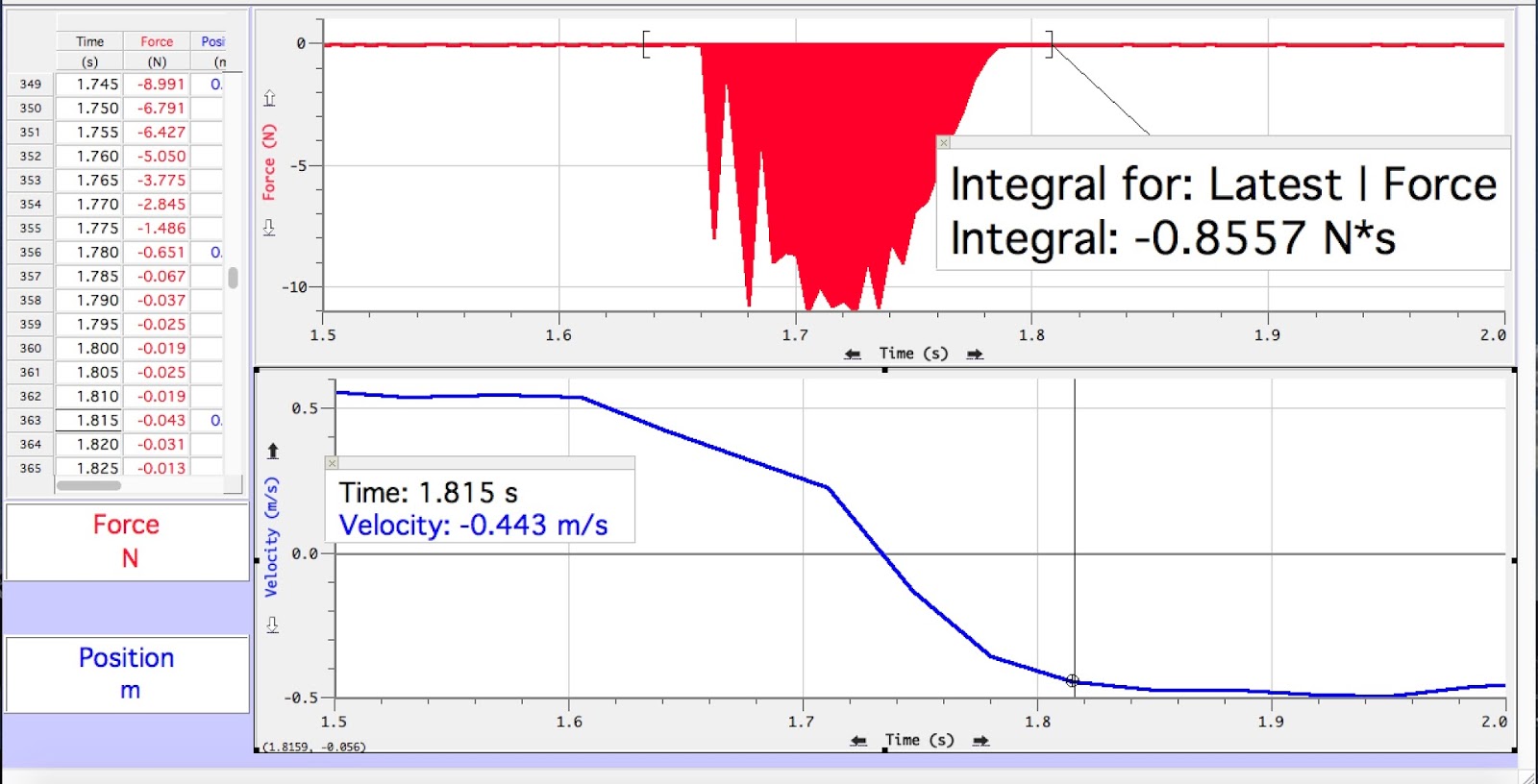Final velocity

Comparison: Our impulse from area under the force vs. time graph was -0.8557 Ns and calculated change in momentum was -0.7674 kgm/s. They are off by 0.08833 or 5.44%, which can be considered not bad comparing to the first two experiments. Comparing the curves we got from experiment 3 with experiment, we saw that the two graphs are similar. 

Conclusion: From all three of our experiment, the first experiment was way too off, the second and the third experiments' results are acceptable since they are less than 10%. We could also see that the results get better. Therefore, the impulse-momentum theorem can hold true. The reasons why we got somewhat large percentage of errors are that our track might not have been re-leveled after each trial. The force sensor or the motion sensor readings can be off. 

17-April-2017: Lab13: Magnetic Potential Energy

Lab 13: Magnetic Potential Energy Lab
May Soe Moe
Lab Partners: Ben Chen, Steven Castro
17-April-2017

Objective: To verify that the conservation of energy applies to the system we came up for this lab.

Introduction: By turning on a vacuum, the air glider would glide along the air track and move toward the motion detector. Two magnets with same polarity at the end of the cart and the air track are attached. Since they have the same polarity, once the glider reaches to the end of the track, the magnet at the end would repel the glider, causing the glider to move to other direction of the motion. In this lab, we would like to show that our kinetic energy and potential magnetic energy of our apparatus is constant, therefore, energy is conserved. The problem of this lab was that we did not have an equation for magnetic potential energy. Therefore, by plotting a graph of Force vs. separation distance graph, we would get the power fit to the graph to get that equation that represents the magnetic potential energy. Once we get our equation for magnetic potential energy, we would use that as our model to figure out if our conservation of energy in our system or set up is conserved or not.

Experimental Procedure:

Apparatus:

Our Apparatus for this lab

 (1) The set up was already done by the professor.

(2) Air glider is used to move along an air track when the air is turned on. There are numerous holes in the air track. Through those holes, air would push up the glider, making it not really in contact with the track. That makes the track frictionless surface.

(3) One magnet was sticked to the end of the glider and another was sticked at the end of the air track. What would happen with this lab is that the glider would move toward the motion detector when air is turned on. When it reaches to the end of the track, the glider would bounce off and move to opposite direction due to the magnets. The magnets have same polarity-- like poles repel, and unlike poles attract each other. Because the magnets' poles are the same, it repelled and let the glider bounce off to other direction. This is almost the same as the spring; the spring would pull back an object when it is stretched to a certain distance and let go.

(4) Here, during the repel, we saw that the glider did not go to the very end of the track nor did it touch the magnet. There was a distance in between two magnets, which we called separation distance r. Like our previous labs before, we would approach this lab to find the force vs. position graph.

(5) We cannot find the force between the magnets directly. Therefore, what we used as a force between the two magnets was by representing force as mgsinθ since the glider was going in the x-direction. We would put the air track at a certain angle by adding books underneath. 

(6) We used bubble level app from our phones to measure the angle of the air track. 

(7) Then how do we get our position? Our position function was the distance between the glider and the motion sensor minus separation distance r between two magnets.

(8) Once we were ready with the setup, we gave a slight push to the glider after turning the air on. We started collecting the data and graphed our force vs. separation distance r graph.

(9) We repeated this procedure a few times by adding books underneath the track to raise the angle. 
And we collected new sets of data at those different angles.

(10) With our collected data, we graphed a velocity vs. time graph, and a position vs. time graph to help us with finding the kinetic energy.

Position vs. Time and Velocity vs. Time graph to help us find Kinetic Energy

(11) We put in all of our datas including our angles and separation distance r values. Then we graphed a force vs. separation distance r graph. 

This is how our force vs. separation of r graph should looks like.

Position and Angle are collected data and Force is calculated data.

How we calculated force for various angles

Our graph of Force vs. separation distance

(12) Doing the powerfit of the force vs. separation distance gave us a function that will represent the magnetic potential energy after doing the integral of this function.

(13) We knew that negative integral of the force and distance function equals to potential energy. Therefore, we integrated the function we got from the graph to get us the function of magnetic potential energy.

Integrating the function from the graph. U represents magnetic potential energy

Verifying the Conservation of Energy

We would try to verify the conservation of energy by putting kinetic energy, magnetic potential energy and the total energy of the system as a function of time onto one graph.

Kinetic Energy, Magnetic Potential Energy and Total Energy in one graph

This is how our Kinetic energy, magnetic potential energy, and total energy should looks like. (standard graph)

Conclusion: By comparing the standard graph and our resulted graph, we can see that they are quite similar, but not constant. We assumed that there was no friction force acting on the glider for our system. But when we assumed there is no friction between two surfaces, the graph should come out like the standard graph. But since it did not come out to be smooth line or curve, we could be sure that there was kinetic friction acting on the glider during the time of glider moving along the track. Although our graph was not smooth, kinetic energy and total energy stayed in that range, without moving up or down too much. Therefore, we can say conservation of energy for our system stayed conserved. 

10-April-2017: Work-Kinetic Energy Theorem Activity

Lab#11: Work-Kinetic Energy Theorem Activity
May Soe Moe
Lab Partners: Roya Bijanpour, Ian Lin
10-April-2017

Objective: To inspect and possibly confirm the statement of the Work-Kinetic Energy Theorem that the work done on a object is equal to the change in kinetic energy.

Introduction: We had done four separate experiments: (1) work done by a constant force, (2) work done by a non constant spring force, (3) kinetic energy and the work-kinetic energy principle, and (4) work-KE theorem. In this lab we wanted to confirm the Work-Kinetic Energy Theorem, which states that the total work done on an object is equal to the change in kinetic energy. We also knew that the area under the force vs. position graph is equal to work done on an object. Therefore, in this lab, we set up our apparatus so that we could get a graph of force vs. position graph, which would give us the work done on an object by finding an integrated value of an area under the graph and the kinetic energy at that position. When the two values we got from the kinetic energy and the integrated value of the graph are equal, we would compare them and see what we can conclude from our results.

Experimental Procedure:

Experiment 1: Work Done by a Constant Force

Apparatus:

The apparatus for first experiment: the string was not very visible in the picture.

(1) We set up our apparatus as above: we used a cart connected with a hanging mass with a string through a pulley. 

(2) Then we made sure the track was leveled, meaning the cart would roll along the track at a constant speed after giving a gentle push.

Leveling the Track

Our total mass of the cart and 500 grams-- We put in this mass in our kinetic energy in the table.

(3) After the setup and leveling, we would calibrate the force sensor by just vertically holding the force sensor at first and set it to zero. And then we would vertically attach the 500 grams mass to the force sensor and set it to 4.9 N. After it was done, if the force sensor described the force or the weight of the mass to be around 4.9 N, we know that the force sensor is calibrated and it is good to go on with the lab.

(4) We added 500 grams to the cart, hanged 50 grams to the end of the string and pull the cart back.

(5) After that we released the cart, started to collect data, and plotted force vs. position graph.

(6) After getting the force vs. position graph, we added a new calculated column for kinetic energy to our table in Logger Pro and added our equation of kinetic energy- KE= 0.5mv^2, where our mass here is 1.177 kg.

(7) Once we got all of this, we integrated the area under the force vs. position graph using Logger Pro to give us the work done on the cart and kinetic energy at the same point.

Getting the integral and Kinetic energy by highlighting a smaller area

Our Graph of Force vs. Position graph with integrated value and kinetic energy: Larger area highlighted

(8) Above is how our graph came out. In our first graph, we highlighted a smaller area and determined the integral value (0.1287 Nm) and Kinetic energy (0.109J). In our second graph, we highlighted a larger area. Our value of work done on an object was 0.1775 Nm and the kinetic energy was 0.150 J.

(9) When we compared the two values: the integrated value of the area under the force vs. position graph and the kinetic energy from the graph at the same point, we saw that the two values were off by 0.0197 in the first graph and  0.0275 in the second graph. Although we repeated the experiment a few times, we got similar results. Therefore, we suspected that there was friction along the track, and part of the errors might be due to the force sensor, which we had to calibrate after every trial because we saw different force readings.

Experiment 2: Work Done by a Non-constant Spring Force

Apparatus:

Apparatus of Experiment 2

(1) We set up our apparatus as above by attaching the spring to the cart and the force sensor while setting the motion detector on the other side of the cart and the force sensor. We made sure the track was leveled after the setup.

(2) We calibrated the force sensor by repeating the steps we did in experiment 1.

(3) We pulled the cart toward the motion detector until the spring is stretched about 0.6 m.

(4) Then we started collecting data for force applied by a stretched spring for 0.6m of distance.

(5) We began graphing the force vs. position graph as we pulled the cart.

(6) Once we got the graph, we integrated the area under the force vs. position graph.

Experiment 2: Work Done by a Non-constant Spring Force= the Area under the graph.

(7) The integrated value from the force vs. position graph is the work done on the cart by a spring force, which came out to be 0.2424 Nm. The spring constant of our spring is the slope of the equation Force=mx+b. It also makes sense that our spring force equation is F=kx. Therefore, the spring constant is 3.511N/m.

Experiment 3: Kinetic Energy and the Work-Kinetic Energy Theorem

Apparatus:

Our apparatus for experiment 3 was set up the same as in experiment 2.

(1) We measured the mass of the cart, which was 0.549 kg.

(2) We added a new calculated column for kinetic energy of the cart. The equation for kinetic energy of the cart KE=0.5mv^2 was put into the Logger Pro to calculate kinetic energy at different points. Here, our mass was 0.549 kg, the mass of the cart.

(3) We calibrated the force sensor again by repeating the steps in experiment 1 and 2.

(4) After calibration, we pulled the cart along the track so that the spring was stretched about 0.6m from its natural length position.

(5) We began graphing when we released the cart and the spring pulled back the cart to its natural length position.

(6) We would then find the work done by the spring force for the displacement of the cart between any two positions by finding the area under the curve between two points. We would also calculate the kinetic energy of the cart be finding directly from the Kinetic Energy Versus Position graph.

(7) For the change in kinetic energy of the cart, we found the kinetic energy between the same two points we used to find for the work done by the spring force.

(8) We calculated the work done by the spring and kinetic energy of the cart at different positions and repeated a few times.

Kinetic Energy at starting point for this area under the graph

Kinetic Energy at end point for this area under the graph

 (9) Below is the calculated value of change in kinetic energy and the integrated value of the area under the graph-- work done.

Conclusion: From the first two rows, we can see that the work done between 0.155m and 0.222m and change in kinetic energy between that two positions are off by 26.9%. The second set was off by 13.9%, and the third set was off by 3.38%. According to the work-energy principle, the total work done by the spring on the cart is equal to the change in kinetic energy. The work done and change in kinetic energy are not quite close to each other.  We speculated that there was some friction between the cart and the track. The force sensor was not functioning well, which might cause the different reading on the graph, because we had to calibrate it after each trial due to incorrect readings. Other factor that might cause error in our experiment was that the level is not leveled since the cart's velocity moved the track every trial.


Experiment 4: Work- KE Theorem

For this experiment, we watched the movie Work KE theorem cart and machine for Physics 1.mp4 in class. In this video, the rubber band was pulled back by using a machine and the force exerted on the rubber band was recorded by an analog force transducer onto a graph. The graph produced was as below. We calculated the total work done by the machine in stretching the rubber band by dividing up the graph into a triangle, trapezoids, and rectangles, and finding the areas under those shapes. We added all of the areas to get total work done.

The graph produced in the video

The values of displacement, time, mass of the cart are from the video.
The velocity and kinetic energy of the cart are calculated.

The total work done calculated from the Force vs. Position graph was 22.3 J. The final kinetic energy of the cart attached to the machine was calculated to be 23.8 J by using the data from the video.

Conclusion: From our all four parts of the lab, we saw that there were quite difference in between the work done and change in kinetic energy. We doubted that this difference was due to the possible friction between the track and the cart, and the unreliability of the force sensor. Despite of our numerous trials of each experiment, we got our best datas within 20 % range. Therefore, in our results and datas, the work done and the change in kinetic energy are not quite equal to each other. If we had a better reliable apparatus, we might have gotten better results. We can say that since other groups' datas turned out that the work done and change in kinetic energy were pretty close unlike ours. 

3-April-2017: Centripetal Force with a Motor

Lab#9: Centripetal Force with a Motor
May Soe Moe
Lab Partners: Ben Chen, Steven Castro
3-April-2017

Objective: To come up with a model that describes the relationship between the angular speed ω and the angle θ that was created with the string attaching the rubber stopper while revolving around the y-axis--the surveying tripod. 

Introduction: After getting the apparatus set up first, we tried spinning the rubber stopper attached to a string with motor. We found that the rubber stopper revolved around the y-axis--the central pole or surveying tripod got larger radius and larger angle θ as the motor spin at a higher angular speed ω. We wanted to know the relationship between the angular speed ω and the angle θ. We would draw up free body diagrams of all forces acting on the rubber stopper during revolution and derive the angular speed ω in terms of angle θ. From our setup, we did not know the angle that was forming during the revolution and the way we came up with to measure the angle was by setting a ring stand with honrizontal piece of paper sticking out. Then we adjusted the ring stand's height so that the rubber stopper will hit the horizontal paper. When we got that height, then we could mathematically calculate the angle with all our other measurements and datas. From our setup, we could calculate the missing values such as the angle θ, the radius created by the string with rubber stopper, the total radius (the original radius of the apparatus and the radius created by the string with rubber stopper) using trigonometry. We would calculate our derived angular speed ω equation using the calculated missing values (θ, total radius). We could then compare the values we got from our derived equation and the angular speed formula which we knew-- ω= 2π/T. 

Experimental Procedure:

(1) The apparatus set up was done by the professor as in the picture below:

Apparatus

Diagram we used for calculating θ, Lsinθ, and Total Radius

(2) The apparatus was set up by putting an electric motor on a surveying tripod, a vertical rod on the motor, a horizontal rod perpendicularly mounted on a vertical rod, a long string tied to the end of the horizontal rod, a rubber stopper at the end of the string, and a ring stand with a horizontal piece of paper sticking out.

(3) We ran the electric motor and let the rubber stopper revolve around the surveying tripod at unknown angular speed ω and angle θ.

(4) We ran the motor at certain angular speed ω and timed the time to complete ten revolutions. And we divided that time by 10 to get the time for one revolution.

(5) We adjusted the ring stand with a horizontal piece of paper sticking out while the rubber stopper was spinning around the tripod to a height when the spinning rubber stopper hit the horizontal paper.

(6) We stopped running the electric motor when the rubber stopper hit the horizontal paper taped to the ring stand. We measured the height of the ring stand from the ground to the horizontal paper.

(7) We also got other measurements such as the Length of R, the length of L, and the length of H as described in the diagram above.

(8) We increased the voltage of the motor driving the system and repeated the same steps for five more times to get our datas.

Calculations:

Calculated Values

Here are the equations that were used to find the values above and some clarifications that might be needed for the column headers.

Here is our free diagram of forces acting on the rubber stopper and our derived equation that represents the relationship between the angle θ and the angular speed ω.

Conclusion: 

We compared the two angular speed ω values we got--values we got from our known angular speed ω equation-- ω= 2π/T, and our derived equation. It turned out that our theoretical values are larger than our experimental values. Our percentage of errors came out to be less than 5% except the last ω. Except our error percentage, our results are in the acceptable range. The last angular speed ω for both using T and using h are very high, thus leading to higher percentage error. Uncertainties or things that led us to commit some errors could be that we assumed the angular speed ω of the string with the rubber stopper was constant throughout the rotation when it could be speeding up over time. We ignored air resistance. The height of the ring stand with horizontal paper sticking out, and the L sin θ values could be smaller than what we recorded in reality, since the rubber stopper hit the horizontal paper when what we should record was the rim of the paper. We took longer time as we had to time the time to complete ten rotations and to adjust the height of the horizontal paper sticking out so that the rubber stopper would hit the paper. During that time of ten revolutions and adjusting the height of the paper, the rubber stopper could be speeding up. Regardless of all the uncertainties and errors, our experimental values came out to be acceptable.

5-April-2017: Activity- Work and Power

Lab#10: Work and Power
May Soe Moe
Lab partners: Ben Chen, Steven Castro
5-April-2017

Objective: To calculate the work and power output produced during performance of activities such as walking up the stairs, running up the stairs, and lifting up a bag of certain mass to a height h that is connected to a rope and a pulley.

Introduction: In our daily lives, we do work and produce power, which in Physics work equals force applied and distance traveled, and power is work divided by time. We can also relate to power in our daily lives, especially as the technology improves nowadays. We use power to produce electricity, to light up our homes, to watch TV, to charge our mobile phones and laptops, and to heat up our food in microwave. We have to use power even to use internet. But we have no idea how much it takes to produce power. Therefore, we tried to do work by walking up the stairs, running up the stairs, and lifting up a bag with mass to a height, which was attached with a rope and a pulley. Using our known formulas of work and power, we would calculate the work done and power output during the activities. Using the same formulas, we could calculate how much it takes to produce power for our everyday activities as mentioned above. In this case, our work done and power output were:

Experimental Procedure:

Part 1:
(1) The professor set up the rope that goes over pulley. At the end of the rope from the ground, three backpacks with different masses (5 kg, 6 kg, and 9 kg) were tied. At the balcony, the pulley was tied to a wooden stick so that it could be used to connect to the rope and the backpack.
(2) During this procedure, we were to lift up a backpack containing a known mass (5 kg,  6 kg, and 9 kg) from the ground to the wooden stick by pulling on the rope that went over a pulley-- tied to a wooden stick at the balcony.
(3) Each individual in the group was to complete the experiment and to get timed for their own since individuals' time to complete the experiment were different depending on the ability and strength to lift the backpack. We could also choose which backpack we wanted to lift up. When pulling up the backpack, one person from the group had to press down the wooden stick that was tied to the pulley so that it would not move up and hurt the people passing by.
(4) My time to lift up the backpack was 49.93 seconds, the backpack I lifted up contained 5 kg, and the height from the ground to the balcony was 4.5 meters.

Lifting up the backpack

Walking up to the stairs

Calculation For Part 1:

The power output to lift up a 5 kg backpack for me came out to be 4.42 Watts. 

Part 2: 

(1) For this part, each individual from the group walked up the stairs and got timed to get to the top of the stairs.
(2) We measured the height of a step of a stair, which was 17 cm or 0.17 m. There were 26 stairs, therefore, the total height was 26 stairs x 0.17m, which came out to be 4.42m.
(3) My power output to reach the top of the stairs came out to be 223.1 Watts.

 Part 3: 

(1) We timed while running up to the stairs. The height of the stairs was the same from part 2. Calculation of my power output to reach the top of the stairs was 441.7 Watts.

Conclusion:

(4a) Q: In our analysis, we neglected our kinetic energy in calculating the total work that we did. Make a reasonable estimate of how big of an error this introduces into your results.
              
Calculation:

Calculating the distance L of a flight of stairs

        My calculations tell me that error of kinetic energy for lifting up the 5 kg backpack was 0.009%, error of kinetic energy for walking up the stairs was 0.6%, and the error of kinetic energy for running up the stairs was 2.4%. All the errors were under 5%, which is in acceptable range, therefore, the negligence of kinetic energy in calculating my total work that I did was not affected.

(4b) Q: A microwave oven typically has a power consumption of approximately 1100 Watts. How many of the flights of stair we used in this lab would you have to climb each second to equal the power output a microwave oven?

Calculation:

(4c) Q: Suppose you are cooking two potatoes in the microwave oven for a total of 6 minutes. How may flights of steps total would you have to climb to be equivalent to the amount of work that it took to run the microwave?

Calculation: 

(4d) A person in reasonably good shape can comfortably put out 100 Watts continuously (say, by riding a stationary bicycle connected to a generator.) A 100 % efficient water heater would require about 12.5 MJ (megajoules - 10^6 joules) of energy to heat water for a 10-minute shower (flow rate of 10 liters per minute, approximately 2.5 gallons per minuter, water being heated from 20 Degrees Celsius to 50 Degrees Celsius.)

(Q1): How much power is this?

Calculation: Power to heat water came out to be 20833 Watts.

(Q2): If you gathered a group of people to ride bicycle-powered generators in order to heat the water for your shower in real time, and each one was putting out 100 Watts, how many people would it require to heat the water for your shower?

Calculation: 208 men are needed to heat the water for my shower.

(Q3): If instead you were going to provide all of the energy yourself, how long would you have to ride on a bicycle-powered generator in order to heat water for your 10-minute shower?

Calculation: I need to ride a bicycle-powered generator for 124998 seconds if in seconds, 2083 minutes if in minutes, or 35 hours if in hours in order to heat water for my 10-minute shower.