15-March-2017: Trajectories

Lab#5: Trajectories
May Soe Moe
Lab Partners: Ben Chen, Steven Castro
15-March-2017

Objective: To predict where the ball that was launched from the top of an inclined board would land.

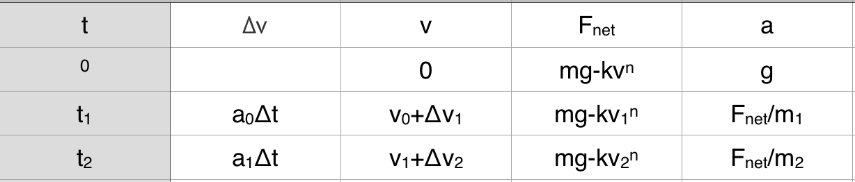
Introduction: The velocity of the objects in projectile motions are calculated separately. We calculate its velocity in x-direction and velocity in y-direction. We knew that the x-velocity and y-velocity are independent of each other and the only relationship between them is time. By finding the time, we can know the position and velocity of the object regardless of being in x or y direction.

Experimental Procedure:

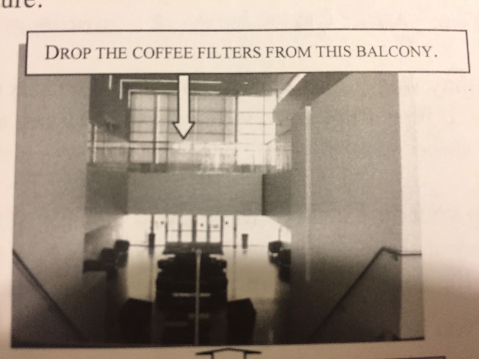
(1) Set up the apparatus as below:

(2) We placed a carbon copy to the floor where we thought the ball would land. We confirmed where it would impact by launching the steel ball as a trial. Then we taped the carbon copy to secure it so that it is not moved by the ball at the time of impact. 

(3) We launched the ball five times from the same launching point. We verified that the ball landed in almost exactly the same place for each time. 

(4) We measured the height of the table+ the height of the block that was put in between the table and the aluminum b-channel. We also measured the distance from the table's edge to the landed position. The measurements were: h=96.3+/-0.1cm or 0.963 +/- 0.001 m, and x=75.5+/-0.1 cm or 0.755 +/- 0.001 m. 

The height of the table+ The height from table to the v-channel

The horizontal distance from the edge of the table

(5) We calculated the launch speed of the ball from our measurements.

Calculation of the launching speed

(6) We added an inclined plane at the end of the table, touching the v-channel. The angle go the inclined board was measured with bubble level from our phones, which turned out to be 49 Degree. In this case, if we launched the steel ball from the same launching point as before, the ball would stroke the distance somewhere along the board. So, we predicted where the ball would land, and confirmed it by trying once before we recorded where it landed on the carbon paper. Once we were satisfied with where it would land, we taped the carbon paper to record the landed position. We also put some weight at the end of the board so that it would not move during the ball's launching period. 

(7) We measured the landed distance. We calculated the theoretical distance from the known angle 49 degree and previously calculated launching speed. 

Calculation of where the ball landed

(8) Once we got the theoretical and experimental values, we calculated the uncertainties of the launching speed, angle, and the distance.

(9) The launched speed was 1.704+/- 0.028 m/s and the distance along the inclined board was 1.055+/-0.331 m. 

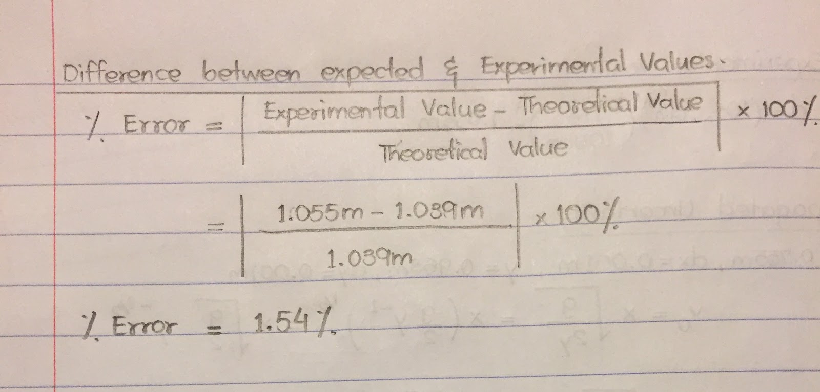
(10) I calculated the error percentage and it came out to be 1.54%, which is within acceptable range.

Conclusion: The error percentage between our experimental value and theoretical value is 1.54%, which is acceptable as the number is not too big. The uncertainties of this lab could result from the measurements of horizontal distance from the table edge, the distance along the inclined board, the vertical distance from the v-channel to the floor, and the angle. What we used to measure all the distances was a meter-stick, which we had rounded to the approximate value. When we measured the angle, we used the phone app, which was not made for experimental purposes. Another error could be  that the board kept moving despite of putting a heavy mass at the foot of the board when the ball was launched. This could result in certain difference of angle. In this case, we neglected the friction force between the surface of the v-channel and the ball. In conclusion, although the theoretical and experimental values of the distance along the board were different, it was within the acceptable range. Through this lab, we learned that the x-velocity and y-velocity during a projectile motion are independent of each other. What relates them is the time. Through the time, we could find out the position, the launching speed and time of the aluminum ball that was in projectile motion.

13-March-2017: Modeling the Fall of an Object Falling with Air Resistance

Lab#4: Modeling the Fall of an Object Falling with Air Resistance
May Soe Moe
Lab Partners: Ben Chen
13-March-2017

Objective: To determine the relationship between air resistance force and speed, and to model the fall of an object including air force and to test out the model.

Introduction/Theory: We wanted to determine the relationship between air resistance force and speed. We did not know air resistance force of an object. But we presumed that air resistance force of an object depends on that object's speed, its shape, and what it is moving through. Therefore, we modeled the fall of an object as a power law:

in which k includes the shape and area of the object. We did not know the air resistance force. So we approached this by finding out its motion, velocity and acceleration through its fall and derived the model to a line equation y=mx+b. We figured out the velocity as the slope (n) and y-intercept was the value of ln (k). The experiment procedure is as follow:

Experimental Procedure:
(1)To get the motion and velocity, we chose to drop coffee filters from the balcony of the Design and Technology building 13 and captured videos of its fall.

(2)We dropped one coffee filter at first, and kept stacking it until it was a total of six coffee filters.

(3)Once we got the videos of the fall of coffee filters, we used Logger Pro to analyze its motion and velocity through the video.

(4)We filled the data into the Microsoft Excel and let the rest calculate it. We created 6 spreadsheets for each trial, increasing mass according to one coffee filter, two, three till six coffee filters.

Equations to put into Excel

mass of 1 coffee filter=0.000872 kg

mass of 2 coffee filters=2*mass of 1 coffee filter=0.001744 kg

mass of 3 coffee filters=3*mass of 1 coffee filter=0.003488 kg

mass of 4 coffee filters=4*mass of 1 coffee filter=0.002616 kg

Mass of 5 coffee filters=5*mass of 1 coffee filter=0.00436 kg

mass of 6 coffee filters=6*mass of 1 coffee filter=0.005232 kg

(5)Using the position and time we got from the video, we graphed the position versus time graph, which we derived as below.

(6)We derived it into natural log formula, so that we could graph it as y=mx+b, in which we knew the slope of the position versus time graph gives us the velocity.

(7) From our derivation, we knew that n was the slope or terminal velocity and y-intercept was ln(k).

Position Vs. Time graph of 1 coffee filter
velocity(slope m)=n=-1.283m/s

Position Vs. Time graph of 2 coffee filters
velocity(slope m)=n=-1.683 m/s

Position Vs. Time graph of 3 coffee filters
velocity(slope m)=n=2.109 m/s

Position Vs. Time graph of 4 coffee filters
velocity(slope m)=n=2.409 m/s

Position Vs. Time graph of 5 coffee filters
velocity(slope m)=n=2.695 m/s

Position vs. Time Graph of 6 coffee filters
velocity(slope m)=n=2.785 m/s

(7) Our model predicted the terminal velocities of various coffee filters as below:

(8) The velocities resulted from our model and the position versus time graphs from the video analysis came out to be pretty close.

Comparison of Velocity from Graph Vs. Velocity from Model

(9) Next was to plot the air resistance force(mg) vs. velocity(v) graph using power fit of Logger Pro. The graph would come out to be a concave up graph, which I forgot to screenshot. When you got the graph and power fit, there would be values of A(the value of k) and B(the value of n). Our recorded value of k was 0.00487 and the value of n was 2.245.

The graph of F resistance vs. Velocity should look something like this.

(10)So, I used Excel to come up with similar graph that represents the air resistance force(mg) vs. velocity graph. In this case, it is ln (mg) vs. ln(v). From our derived equation of ln(mg)=n*ln(v)+ln(k).

Ln(mg) Vs. ln(v) Graph

Conclusion: Comparing the velocities of coffee filters from our model and graphs, it came out to be pretty close to each other. The air resistance force from our graph came out to be F_resistance=0.00487v^2.245.

6-March-2017: Propagated Uncertainty Lab

Lab#6: Propagated Uncertainty

May Soe Moe

Lab Partners: Ben Chen, Steven Castro

6-March-2017

Objective: To learn using caliber and to calculate the propagated error in density measurement

Introduction: There are random errors when we measure things, things that we cannot control. We cannot know its exact measurement such as mass, weight, and height of objects. We expect them to be off by several decimals, give or take. In the case when we know we will make errors during our labs, we will calculate how much our error and uncertainty should be. The goal of this lab was to know the uncertainty of our measurement of density through calculations of propagated uncertainty. We calculated uncertainty by doing partial derivatives of our known equation. For this lab, we learned how to use calipers, which can let us measure to two decimal places. We used calipers to measure the height and diameter of two cylindrical metals: Zinc and Aluminum. We also used electric balance to measure the mass of the metals. And we computed the volume and density of each metal, which we found partial derivatives of the equation Density= Mass/ Volume.

Experimental Procedure:
(1) We measured the mass of two metals using electric balance and recorded it.

Measuring the Mass of the Metal Using Electrical Balance

(2) We measured and recorded the height and diameter of two cylindrical medals using caliper. 

Measuring Device- Caliper

             

(3) We calculated volume and density using the recorded data and our known equations of volume and density.

Recorded Data and Calculating Volume and Density

(4) Once we got our density and volume values, we calculated their uncertainty by finding partial derivatives as below:

Conclusion:

Here is the uncertainty values we got from calculation:

6-March-2017: Non-Constant Acceleration Problem(Elephant)

Lab#3: Non-Constant Acceleration Problem
May Soe Moe
Lab Partners: Ben Chen, Steven Castro
Date Performed: 6-March-2017

Objective: To find out the distance of the elephant before coming to rest by numerically and analytically and compare the results

Problem with Given Information

Theory/Introduction: We were given the problem, where we wanted to find out how far the elephant goes before coming to rest, meaning we want to find the distance x when the final velocity v is zero. We knew the following information: the mass of the elephant on frictionless roller skates (5000-kg), the velocity of the elephant (25 m/s), the mass of the rocket on the elephant's back (1500-kg), the rocket's thrust (8000N), and the function m(t)= 1500kg-(20kg/s)*t. In order to figure out the distance, we will approach this problem analytically and numerically. For analytical approach, the professor already did a bunch of calculus, integrating, to find the velocity and position function from Newton's Second Law, Fnet=m(t)a. To numerically approach, we used Microsoft Excel to put in the known values and find what we do not know to figure out the distance that we are looking for. We tried to figure it out by letting the Excel calculate the data and see when the velocity is zero from the spreadsheet. Then we compared what we got analytically and numerically. 

Summary:

(1) We put in the known values from the given problem into Microsoft Excel: M0=6500 kg, v0= 25m/s, b(burning fuel rate)=20kg/s, Fnet= -8000N. We will set Delta t to be 1 second at first and calculate the acceleration, change in velocity, velocity, change in position, and position at each time interval.

(2) What we wanted to find out was the distance the elephant traveled when its final velocity is zero. Since we don't know when the elephant is at rest, we tried to figure out the time when the velocity is zero by filling down the row. 

(3) The concept behind is that we wanted to find out the time it took for the elephant to come to rest because we were using trapezoidal rule to approximate the distance. By making the time interval smaller, the trapezoid gets smaller and it makes accurate approximation of the distance.

How we got the equation for Change in Velocity. 

How We Got the equation for Change in Position.

(4) After filling down the rows, we tried to see when the velocity was zero during the 1 second time interval.

(5) When the time interval is 1second, we saw that the velocity changed from 0.90392744m/s at t=19s to -0.405405m/s at t=20s. This means that the velocity reached zero between t=19s and t=20s. 

(6) As we wanted to get better understanding of exactly when the velocity is zero, we changed the time interval to 0.1s.

(7) We saw that velocity changed from 0.11888376m/s at t=19.6s to -0.0121135m/s at t=19.7s, which gave us more accurate time period and the change in velocity than when time interval was 1 second.

(8) We tried to make Delta t smaller by putting 0.05 second instead of 0.1 second to see how much difference it made.

(9) From the screenshot, we could see that the velocity must be zero in between t=19.65s and t=19.7s since the velocity went from +0.05339083m/s to -0.0121131m/s. 

Conclusion:

(1) When we compared the results we got from doing the problem analytically and doing it numerically, we could see that it was pretty much the same. Analytically approach got us the distance x to be 248.7m. When we did the problem numerically, we plugged in time intervals to be 1second, 0.1 second, and 0.05 second. We got the distance x of 248.628m when delta t was 1 second, 248.698m when delta t was 0.1 second and 0.05s. 

(2) How we know when the time interval we chose for doing the integration is "small enough" is when delta t stops changing the distance x's value. When delta t is small enough, the distance's value will stay pretty much the same to several decimal places.If we didn't have the analytical result to which we could compare our numerical result, we could tell the distance by calculating standard deviation and see in what range we fall into, and to what percent we can be confident that we got the right answer.

(3) We did the same steps as above to figure out how far the elephant would go if its initial mass were 5500kg, the rocket mass is still 1500 kg, but now the fuel burn rate is 40kg/s and the thrust force is 13000N. We changed its delta t to be at 1 second, 0.1 second, and 0.05 second and got the distance x to be 164.021m, 164.034m, 164.034m respectively.