1-March-2017 Determination of g and Statistically Analyzing Data

Lab#2- Free Fall Lab
May Soe Moe
Lab Partners: Ben Chen, Steven Castro
1-March-2017

Objective: To be able to determine and corroborate the validity of the statement that acceleration of an free falling object-- acceleration due to gravity-- without other external forces will always be 9.8 m/s^2.

Theory: Our objective was to determine whether acceleration of all freely falling objects is 9.8m/s^2 as it is stated. To determine it, we did not have a measuring device for acceleration unlike we have balances for measuring weight. Therefore, we determined the motion of the falling object by using spark generator and spark-sensitive paper tape, and an electromagnet. We put a paper taped in between the vertical wire and vertical post of the device. And we got the data marked by sparks as the spark generator created during the time the electromagnet fell onto the ground. After we got the motion, we used the Microsoft Excel to calculate the time, change in distance, mid-interval time, and mid-interval speed. Once we got the numbers, we graphed the velocity versus time graph to provide us with the acceleration due to gravity, which is the slope.

Experimental Procedure: For this experiment, we did not do the whole procedure ourselves as we had only one apparatus. We had to use the spark-sensitive paper that was used during the experiment done by the professor. But the professor demonstrated the procedure. The procedure was as below:
1) We taped the spark-sensitive paper between the vertical wire and the vertical column of the 1.5m
    long device. The electromagnet is held at the top of the device.
2) Once we thought it was ready, we turned on the spark generator and let the electromagnet fall to
    the ground. By letting the electromagnet that is held at the top of the device fell between the
    vertical wire and the device, the spark generator recorded the motion of the electromagnet on the
    spark-sensitive paper tape during its free fall.

Our apparatus for this lab

3) After that, we got the paper that was marked by sparks during the fall and measured the distances
    between the marks with the two meter stick. We recorded the measured distances and input into the
    Microsoft Excel and let the Excel to calculate the time, change in distance, mid-interval time, and
    mid-interval speed.

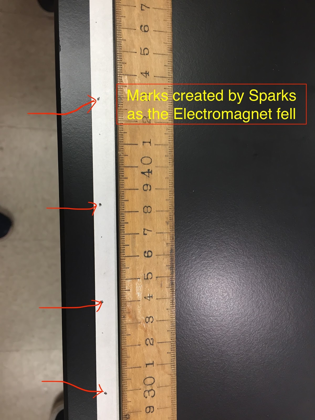
We measured the distances between those marks.

Data Calculated Using Microsoft Excel

4) Then we graphed using the data we got from Excel.
 

5) We also got the function of position by graphing the distance versus time graph using polynomial 

    fit. We knew that the concavity of the position versus time graph tells us about its acceleration, and

    that the slope tells us about the velocity.

Analysis: 
1)

For constant acceleration, we know that v=v0+at. We can see that the velocity of mid-time interval and the average velocity are the same from our derivation.

2)We got the function of velocity-y=9.626x+0.5247 by graphing the mid-interval speed versus mid

   interval time. Since acceleration is the slope of the velocity versus time graph, we could find that

   the average acceleration due to gravity that we got from our data was 9.629 m/s^2 from this graph

   and the linear fit equation. Comparing with our accepted value 9.8 m/s^2, we found that it is off

   by 0.19, which is pretty close.

3)The function we got from the position versus time graph, y=4.7697x^2+0.6901x+0.0103 is in

   the same format as one kinematic equation that we know of: y=y0+v0t+(1/2)at^2. According to

   this graph, our (1/2at^2) is 4.7691, which means our acceleration from this is 4.7691*2=9.538. It

   is off by 0.26. 

Errors and Uncertainty: During this lab, we saw that the position dots on the paper as marked by sparks were different for each paper. So, we knew that the apparatus we used do not give us the same results every single time. Therefore, we tried to use statistical tool to analyze our data. The professor collected accelerations got by all groups and calculated the standard deviation by using the root-mean-square average. It came out that our average acceleration due to gravity was 962.85 and our standard deviation is 10.01. 

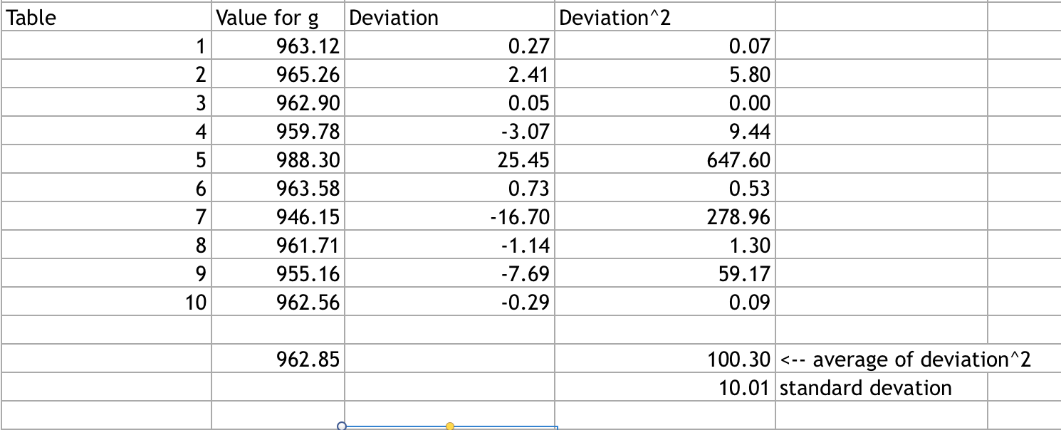
• We found that most of our values of g were too low.
• When we compared our average value with the accepted values, we found that it is off by 0.2m/s^2.
• Most accelerations from different groups came close to 9.5/9.6 m/s^2. 

Conclusion: During this lab, there were random errors, since we did the experiment the same way but got different results/ different position dots on the papers marked by sparks. Our measurements between distances had uncertainties by +/- 0.1cm since we used two meter stick, which could only give us two digits of certain value. One of the systematic errors for this lab is neglecting friction. The acceleration of the electromagnet is big enough and we did not include friction and its effects on our data in this lab. Through this lab, we learned how to calculate standard deviation, which tells you how confident you can be about your data. We learned that we can check our data and compare with other groups' data if we have multiple trials of the lab. Through the diversities of the data, we can find the average and see if the average data comes out to be accurate and precise. We have no way of knowing nor confirming the true value of acceleration due to gravity is 9.8m/s^2.

Therefore, this is a good way to see if our data is accurate and precise by comparing it with other groups' data. We can be confident that it is accurate and precise if all the data are pretty close and also by doing standard deviation. 

27-Feb-2017: Deriving a Power Law for an Inertia Problem

Lab #1: Finding a Relationship between Mass and Period for an Inertial Balance
May Soe Moe
Lab Partners: Ben Chen, Steven Castro
Date: 27 February 2017

Objective: We will try to find a relationship between mass and period for an inertial balance through this experiment. 

Introduction: When trying to find a relationship between mass and period, we want to know the inertial mass--independent of gravity--by using an inertial balance, a device that can be used to measure the inertial mass without depending on gravity. By using an inertial balance, we will be able to figure out the oscillation period of the inertial pendulum for various masses that we will use throughout the experiment. Once we get the measurements of the oscillation periods for different masses, we can develop a mathematical model that represents the relationship between period and added mass (mass of different objects used during the experiment+mass of the tray). After we produce a mathematical model, which is power law in this case, we can use that model to determine the unknown masses of the various objects that are used in this experiment.

Experimental Procedure:

(1) First, we set up the inertial balance by using a C-clamp to secure to the table so that the balance     can oscillate horizontally. After that, we put a thin piece of tape on the end of the inertial balance in order to figure out the period of oscillation.

(2)We set up the photogate by giving it enough space in between the tape and the photogate so that the beam of the photogate can capture the oscillation period. 

We set up the LabPro by plugging into a power source and to computer, which will allow to record the measurements. We used the Logger Pro application to help with the graphs and getting measurements.

(3) Record oscillation periods by adding 100g mass each time on the balance and pulling back the balance until 800g of mass. 

(4)  Create a data table as above in a new Logger Pro document. Add three more columns in the data table-- m+Mtray, ln T, and ln (m+Mtray). 

(5) In order to develop a mathematical model for mass vs. period, we will use the power law:

          T=A [m(added)+M(tray)]^n, and derive it to

      ln T=n*ln[m(added)+M(tray)]+ln A, so that the model will be in a linear equation form--y=mx+b.

      By deriving it, we can find values of A, Mass of the tray and n. 

(6) We can graph a ln T vs. ln[m(added)+M(tray)] and find out the slope( the value of n) and y-intercept (the value of ln A), which will help with finding out the mass of various objects. 

(7) Since we want the graph to be in a linear or straight line, we want the correlation coefficient( which you can check from the graph using linear fit) to be as close as 0.9999. In order to do that we will guess the mass of the tray, which will give us the correlation 0.9999. 

ln T vs. ln(m+Mtray) graphs looks as in above picture by adjusting the Mtray to be 253g, 269g, 280g.

(8) After trials of adjusting the mass of the tray, we get the minimum, intermediate, and maximum values of the mass of the tray that gives us the correlation closest to 0.999.

     M(tray) minimum value=253 g

     M(tray) intermediate value=260 g

     M(tray) maximum value=280 g

(9) Record the values of the slope and y-intercept you get after plotting the graph and adjusting the mass of the tray to be 253g, 260g, and 280g respectively. We use linear fit to give us those values.

(10) We find oscillation periods of two other different objects-- a cellphone, and tape dispenser by putting it on the inertial balance. 

Photogate collects the period of oscillation for different objects as in above picture.

(11) After recording the two new oscillation periods for the cellphone and tape dispenser, we will use the derived power law formula to find the masses of those two objects by plugging in the slope as n, y-intercept as ln A, the two new periods recorded as T, and also the adjusted masses of the mass of the tray. We will solve three different times for the different masses using the minimum, intermediate, and maximum values of the mass of the tray. 

Calculation of the two masses by using the minimum value of the mass of the tray, slope and y-intercept from the ln T vs. ln (m+Mtray) graph

Calculation of the two masses by using the intermediate value of the mass of the tray,
slope and y-intercept from the ln T vs. ln (m+Mtray) graph

Calculation the two masses by using the maximum value of the mass of the tray, slope and y-intercept from the ln T vs. ln (m+Mtray) graph

(12) We also measure the mass of the cellphone (158g) and tape dispenser (688g) by using electronic balance.

The calculated masses of the cellphone and the tape dispenser 

Conclusion: We tried to find the relationship between mass and period by using inertial balance. We recorded the oscillation periods for 100g to 800g. We created a table and plotted it in order to get the values for A and n, to theoretically find out the unknown masses of different objects. The formula used here was T=A*[m(added)+M(tray)]^n, and mass and period are directly proportional to each other by the formula. But we used the derived formula ln T= n*ln[m(added)+M(tray)]+ln A to make it in the straight line formula y=mx+b. When graphing, ln T vs. ln (m+Mtray) came out to be a straight line, which let us know that n was the slope, and y-intercept was the ln A, according to the formula. We collected different periods for two other objects--cellphone and tape dispenser-- and calculate the theoretical masses of the objects. The calculated masses came out to have different values, which are not close to the actual masses of the objects, when compared to the actual masses from the electronic balance. 

Errors: There may be errors that led us to get different values for theoretical masses and actual masses. We could have used different forces for each time to pull back the balance when recording oscillation periods for different masses. We assumed that forces to pull back the balance are equal, which could make a difference in comparing masses. The actual measured mass from electronic balance could actually be weight, including the gravitational mass.